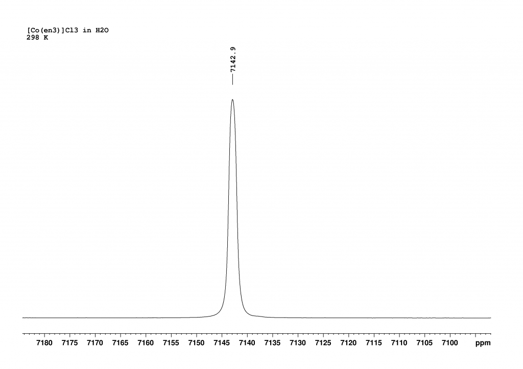
After seeing the spectacular 59CO spectra of [Co(en)3]3+in D2O,1 I thought that this could be improved upon. The impetus for this came from papers by Borer et al.2 and Iida et al.3 that described the spectroscopic differentiation of the two enantiomers of the complex using sodium tartrate and 59Co NMR spectroscopy. Firstly, I recorded the 59Co NMR spectrum of [Co(en)3]3+ in H2O. This revealed a single peak, which combined the signals of the two enantiomers (Δ and Λ isomers in a ratio of 1:1).
59Co spectrum of [Co(en)3]Cl3 dissolved in H2O at 298K. The spectrum was recorded using a 700 MHz NMR spectrometer operating at a frequency of 163.2 MHz.
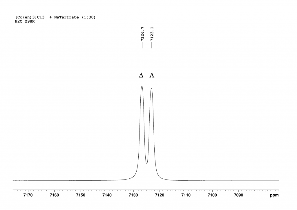
The addition of L-(+)sodium tartrate has a surprisingly clear effect. The original peak splits into two new peaks that are shifted to higher field.
Excess L(+)-sodium tartrate produces two peaks, which correspond to the presence of two enantiomeric complexes. The peak at 7123.1 ppm corresponds to the Λ-isomer and the peak at 7126.7 ppm corresponds to the Δ-isomer.
Deconvolution of the two peaks shows that they are in an integrative ratio of exactly 1:1. The cause of the splitting in solution lies in the formation of contact ion pairs, which behave like diastereomers in solution and thus result in separate 59Co signals for each enantiomeric complex.3 Part I of this post reported that the complex [Co(en)3]+ forms isotopomers when dissolved in D2O through H/D exchange, all of which exhibit their own 59Co NMR signal. This naturally raised the question of what would happen if D2O was added to the solution of the complex in H2O with sodium tartrate. I hoped that each signal from the two enantiomers would be further split into the corresponding isotopomers. To my great delight, this is exactly what happened. The resulting spectrum is one of the most spectacular spectra I have ever measured.
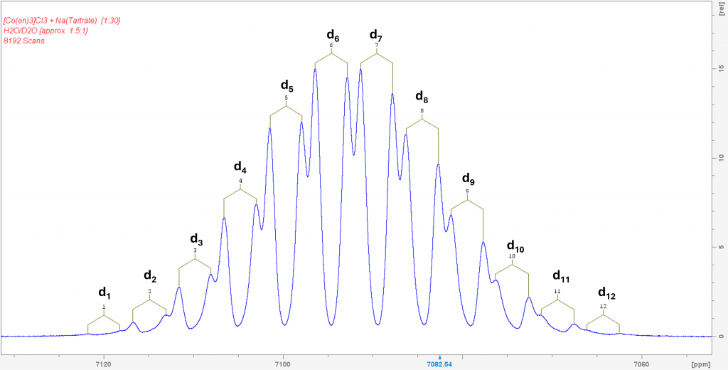
59Co spectrum of a mixture of [Co(en)3]Cl3 with excess sodium tartrate in H2O/D2O (approx. 1/1.5). The 24 peaks are caused by the splitting of the 12 possible isotopomers (d1 to d12) into the signals of both enantiomeric complexes(Λ and Δ-isomer).
This spectrum was obtained by recording 8192 scans in order to extract the signals of the low-concentration isotopomers d1 and d12 from the noise. The two signals of the isotopomer d0 are missing because its concentration is so low that its signals are lost in the noise. The spectrum shows the isotopomers in equilibrium. Even after 7 days, it remains unchanged. This means that the isotopomer distribution can ultimately be controlled via the H2O/D2O ratio, which is also reported in the literature. To be honest, I was lucky to have hit the H2O/D2O ratio in such a way that the isotopomers d6 and d7 form the maximum.
14N NMR of [Co(en)3]3+
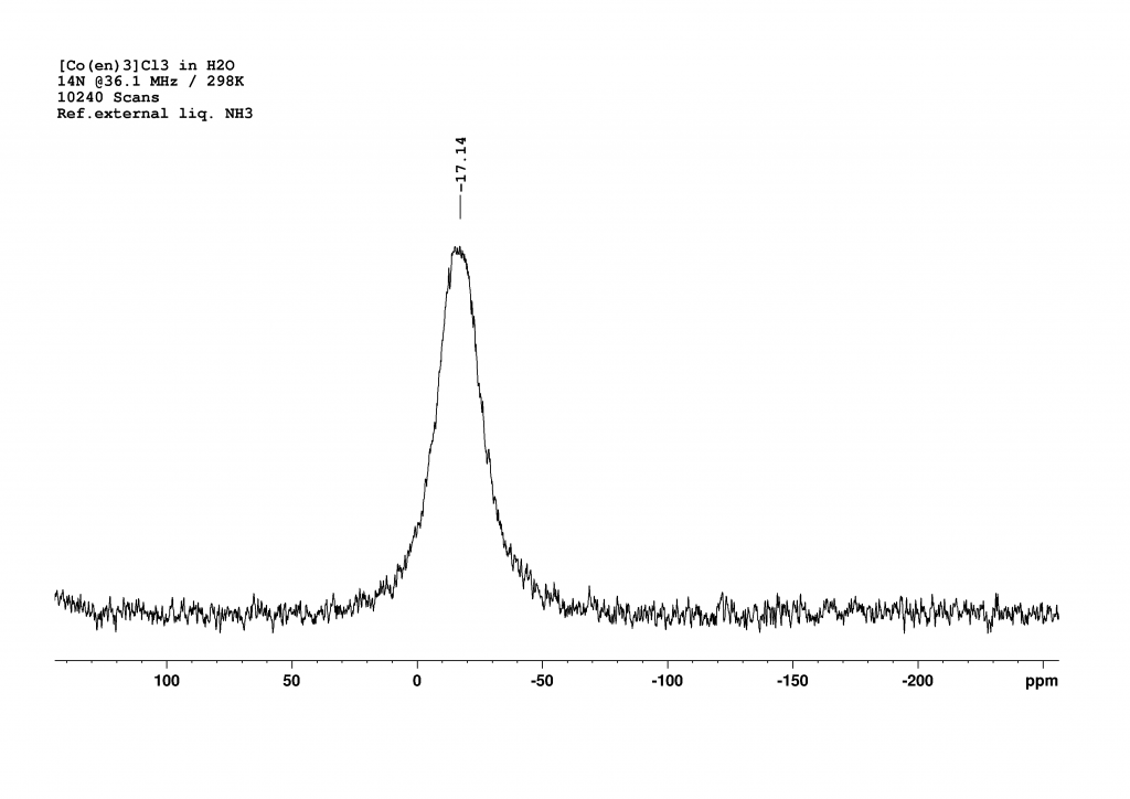
To complete the investigation of [Co(en)3]3+, it seemed sensible to record a nitrogen NMR spectrum. All my attempts to produce a 15N-HMBC spectrum failed miserably. The ligand’s protons produce relatively broad peaks in the 1H NMR spectrum, which probably prevents polarisation transfer to the 15N atoms. I was also unable to find any 15N data in the literature. The last option was therefore 14N NMR spectroscopy. Fortunately, the appropriate measuring head on our 500 MHz spectrometer had recently been repaired, enabling us to carry out the measurements promptly. Since the signals from primary amines typically appear in the range of 20 to 30 ppm (reference fl. NH3 = 0 ppm) and no dramatic shift was expected due to the coordination of ethylenediamine on cobalt, we searched in a window around this range and were rewarded with a broad signal at -17 ppm.
14N NMR of [Co(en)3]Cl3 in H2O.
A measurement time of 48 minutes (10240 scans, with a relaxation delay of 0.01 s and an acquisition time of 0.28 s) was necessary to obtain a good spectrum. The peak is very broad (FWHM = 720 Hz), which is unsurprising given that the nitrogen atoms are not symmetrically surrounded. I was somewhat surprised that the nitrogen atoms are more strongly shielded than in the free ligand. I currently have no explanation for this.
25 years ago, Peringer et al. published a paper entitled “1J(199Hg199Hg) values of up to 284 kHz in complexes of [Hg–Hg]2+ with crown ethers: the largest indirect coupling constants”.1 It reports on the extremely large scalar coupling constants between non-equivalent directly bonded mercury atoms. Unfortunately, the communication was not followed by a full paper.2 In this post I would like to address some questions that have remained unanswered and explain in more detail how the authors calculated the coupling constants of the mercury atoms. Perhaps this will motivate someone to repeat the experiments in order to clarify the questions. I think there is still plenty of room for interesting discoveries. The reaction of a simple Hg2+ salt with elemental mercury and subsequently with the ether 18-crown-6 leads after crystallization from dichloromethane to the complex cation {[Hg2(18-crown-6)2(dmso)(μ-dmso)]}24+(complex 1). The structure of this cation is shown below.
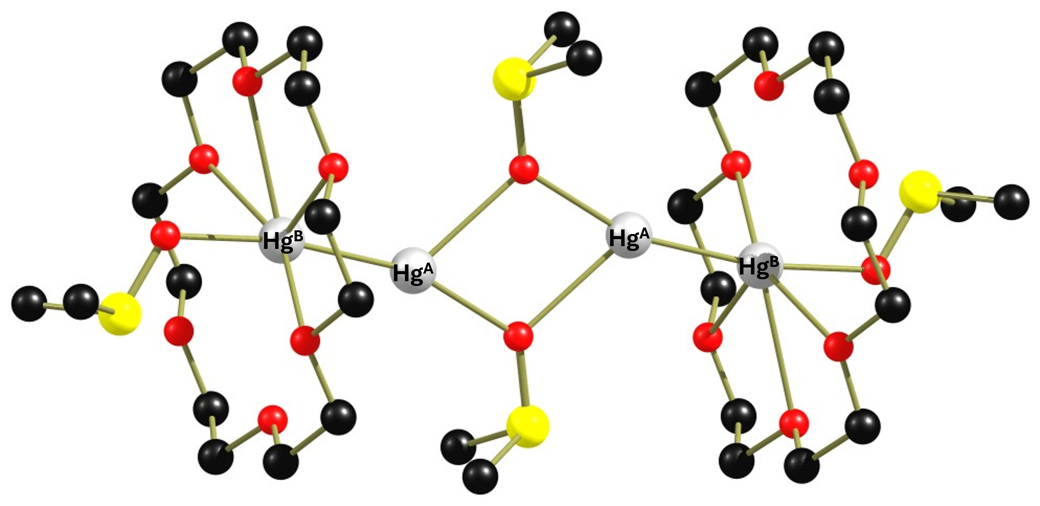
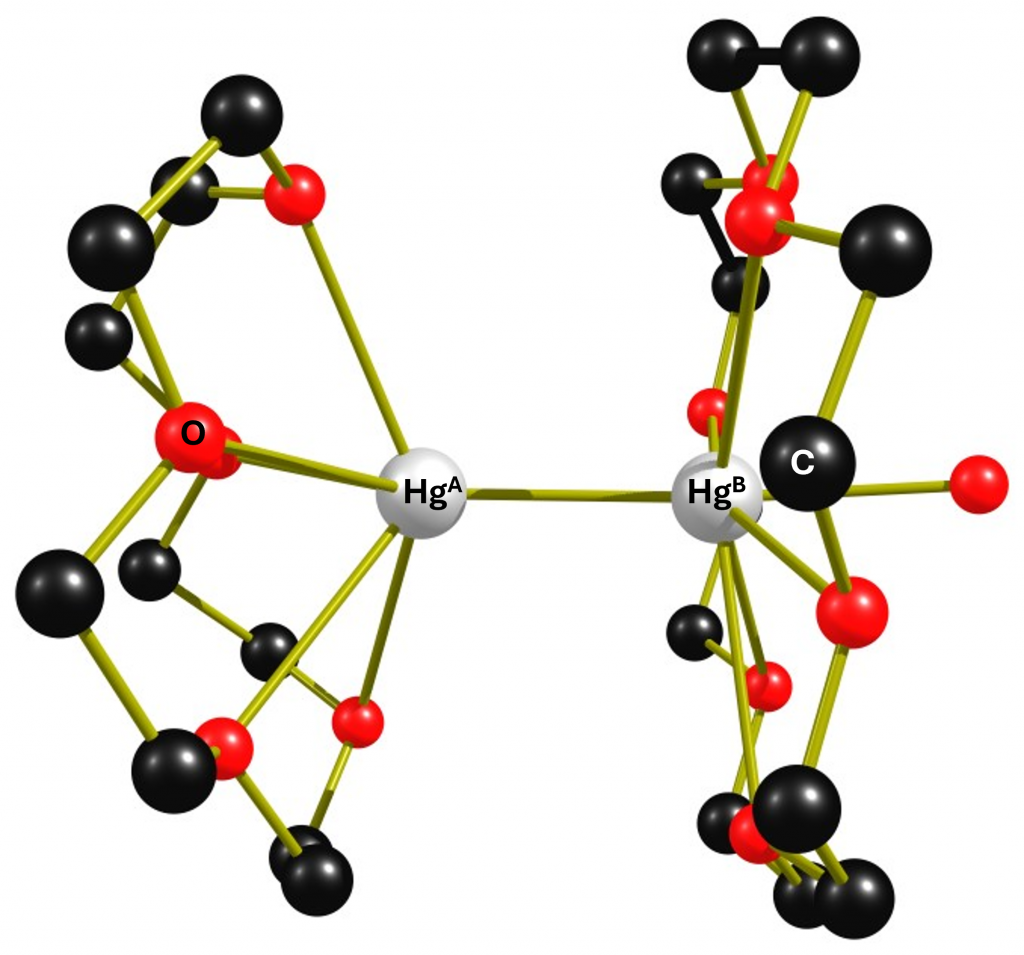
Figure 1: Molecular structure of complex 1. The distance HgA-HgB is 2.5218(7) Å. The Hg-O distances for 18-crown-6 vary between 2.719(6) Å and 3.042(6) Å.
The dimeric complex 1 is highly interesting because it contains two non-equivalent Hg(+I) atoms that are linked to each other via an Hg-Hg bond and will therefore couple with each other in the 199Hg NMR spectrum. Before we look at the NMR spectrum of the compound, I would like to discuss a detail in the structure of complex 1 that is important for the spectra. Of the six Hg-O distances, four are in the range of 2.7 Å to 2.8 Å and two are in the range of 3.0 Å, which is already larger than the sum of the van der Waals radii of mercury and oxygen. Therefore, in figure 1, two oxygen atoms have no coordinative bond to the mercury atom. The original paper was more generous. In any case, the large differences in the Hg-O distances indicate that the crown ether binds fluxionally. Unfortunately, neither 13C nor 1H NMR data were given in the paper, so no statement can be made about the dynamic behaviour of the ligand. Only one 199Hg spectrum (reference HgO/HClO4) was recorded at 243 K in non-deuterated dichloromethane, showing 4 signals.
Insert: NMR spectra of AB spin systems
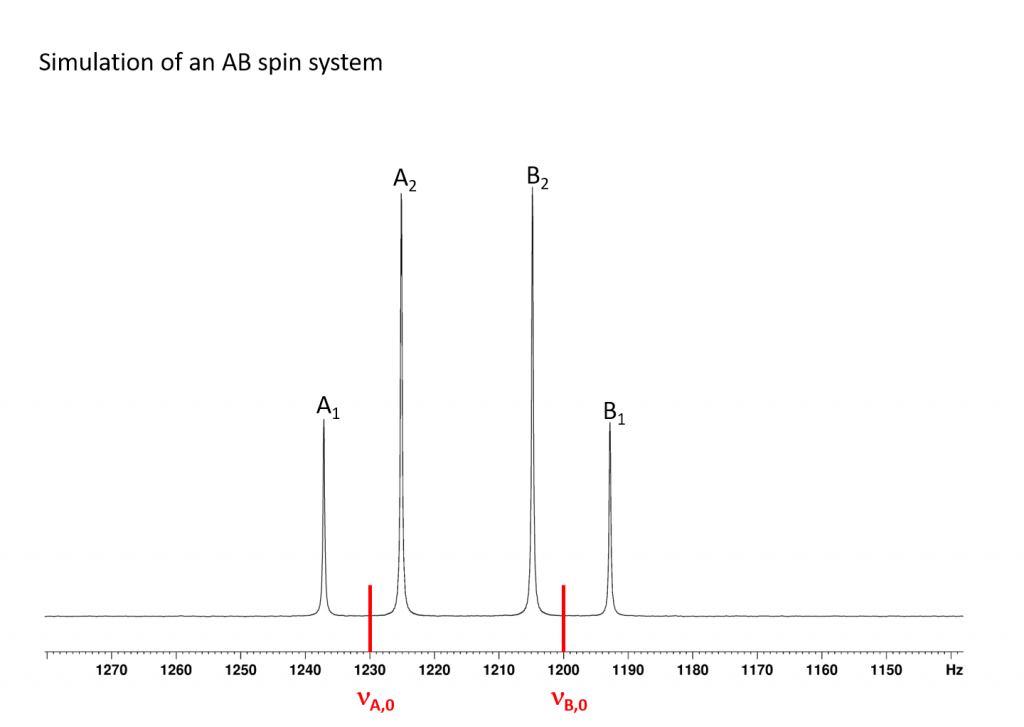
If the coupling constant JAB of two atomic nuclei A and B is in the range of the difference between their Larmor frequencies (Δν=νA-νB), the phenomenon of strong coupling occurs and this is referred to as an AB spin system. If the difference between the Larmor frequencies is significantly greater than JAB (at least more than 10 times), this is referred to as a first-order spectrum and an AX spin system is present, which shows two simple doublets in the spectrum according to the n+1 rule. The NMR spectrum of an AB spin system typically looks like the one shown in the next figure.
Figure 2: NMR spectrum of a typical AB spin system(Δν=3 JAB).
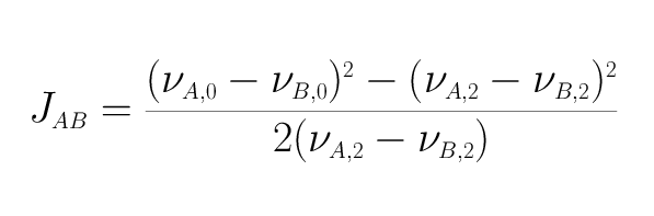
The spectrum shown is typical of an AB spin system. Compared to the AX spin system, the two doublets are distorted. The inner transitions (A2 and B2) are much more intense than the outer transitions (A1 and B1). It should also be noted that the Larmor frequencies (νA,0 and νB,0) of the nuclei are no longer in the centre of the doublets, but are shifted towards the more intense transition. As Δν becomes smaller, peaks A1 and B1 become smaller and A2 and B2 become larger. In terms of the 199Hg spectra discussed below, this means that the A1 and B1 transitions become so small that they are lost in the noise of the spectra, so that only the A2 and B2 peaks can be detected. At first sight, one might think that the coupling constant JAB can no longer be determined. After all, it is calculated very simply from the difference νA,1-νA,2 or νB,2-νB,1. However, if you know the position of νA,0 and νB,0, there is another way to calculate the coupling constant JAB. The corresponding equation is
It can be derived from the basic equations3 that describe the frequency positions in an AB spin system.
199Hg NMR spectrum of complex 1
The spectrum of complex 1 is not shown in the original paper. However, it can be reconstructed from the given data by means of simulation. The spectrum was measured at 243 K in CH2Cl2 at 53.63 MHz (i.e. on a 300 MHz NMR spectrometer). The chemical shift of HgA is 944 ppm and that of HgB (complexed to 18-crown-6) is 435 ppm. At this point, I would like to point out that the authors do not explain how they arrived at this signal assignment. The coupling constant 1JHgHg is an incredible 220300 Hz (± 790 Hz). The spectrum then looked something like this:
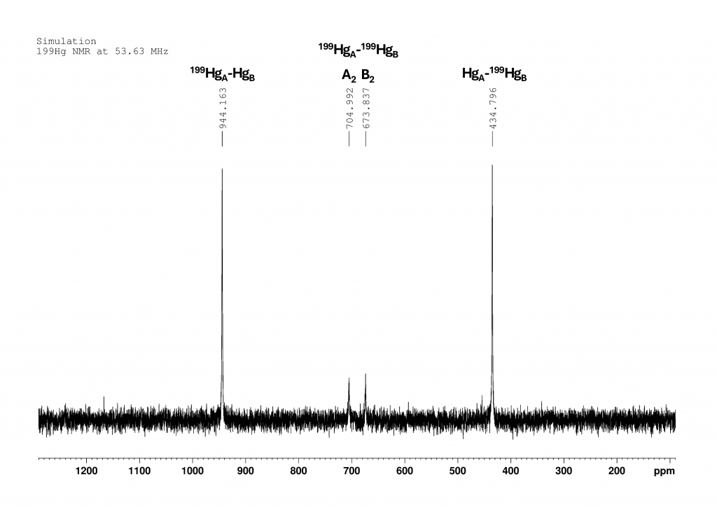
Figure 3: Simulation of the 199Hg NMR spectrum of complex 1 according to the data from Peringer et al..1
The two large peaks show the signals of 199HgA bound to a non-active Hg (944 ppm) and 199HgB bound to a non-active Hg. The two small peaks in the center belong to the two doublets that are formed by the coupling of two 199Hg atoms. They correspond to peaks νA,0 (705 ppm) and νB,0 (674 ppm) from Figure 2. There are 7 stable mercury isotopes. Only the isotope 199Hg (natural abundance 16.94% 5) is accessible in liquid using NMR spectroscopy. If we look at complex 1, there are 10 isotopomers to consider for the spectrum. In the following list, all 199Hg atoms are labeled with Hg and all other Hg isotopes are summarized under the symbol Hg.
Only isotopomer 1 does not give a NMR signal. Since the measured 199Hg NMR spectrum provides only four signals of very different intensities, it is reasonable to conclude that 199Hg atoms not directly bound to another 199Hg atom exhibit a single resonance for both HgA and HgB. These resonances correspond to the νA,0 and νB,0 positions shown in Figure 2. The intensity of these signals is directly proportional to the abundance of 199Hg in positions A and B, respectively.6 We then expect the intensity ratio of the four peaks to be approximately 5:1:1:5, with roughly comparable line widths in the spectrum shown in Figure 3.
When complex 1 is reacted with two equivalents of 15-crown-5 in CH₂Cl₂, it degrades to form the dinuclear complex [(15-crown-5)Hg-Hg(18-crown-6)(dmso)]2+ (2). This cocrystallises with complex [(15-crown-5)Hg-Hg(18-crown-6)(H2O)]2+3 when an attempt is made to isolate it. However, it is possible to spectroscope complex 2 cleanly in solution. I have isolated the structure of complex 3 from the corresponding cif file, which is shown below. I have dispensed with complex 2 because some of the carbon atoms in it are so strongly disordered that its representation becomes very confusing.
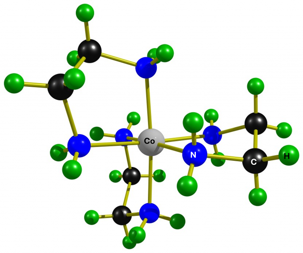
Figure 4: Structure of [(15-crown-5)Hg-Hg(18-crown-6)(H2O)]2+3. The structure of complex 2 is analogous. Only the terminal H2O is substituted by a DMSO molecule.
All distances are in the range of the sum of the van der Waals radii of oxygen and mercury, but the high variance with differences in the distances of 0.3 Å and 0.8 Å, respectively, strongly indicate that the crown ethers in solution should show a pronounced fluxional behavior. Unfortunately, the authors do not provide any 1H or 13C NMR data, so the dynamic behaviour of the ligands cannot be verified.
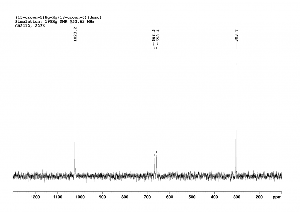
The 199Hg NMR spectrum of complex 2 in CH2Cl2 at 223K is analogous to the spectrum of complex 1 (Figure 2). It does not add much value, but I simulated and plotted it anyway so that the reader does not have to scroll up constantly.
Simulation of the 199Hg NMR spectrum of [(15-crown-5)Hg-Hg(18-crown-6)(dmso)]2+2. The assignment of the peaks is analogous to Figure 3. The signal at 304 ppm belongs to the Hg atom bound to 18-crown-6. The peak at 1023 ppm belongs to the Hg atom bound to 15-crown-5. The two small peaks in the middle belong to the two doublets resulting from the strong coupling of the two inequivalent mercury atoms.
In this case, the coupling constant is calculated as 263200 Hz (±590 Hz). But that’s not the end of the story. The record-breaking result is obtained when complex 1 is dissolved in methanol. In this case, an equilibrium between [(15-crown-5)Hg-Hg(18-crown-6)(dmso)]2+2 and [(15-crown-5)Hg-Hg(18-crown-6)(MeOH)]2+4 forms in the solution. Unfortunately, the authors do not comment on the position of this equilibrium. Nevertheless, analysis of the 199Hg NMR spectrum of this mixture reveals a 1JHgHg coupling constant of 284100 Hz(±860 Hz) in 4, which is the highest coupling constant recorded to date. Unfortunately, 4 could not be crystallised. Instead, mixed crystals of 2 and 3 were obtained. The water had diffused from the air into the methanol during crystallisation, which did not take place under protective gas.
Loose ends
It is in the nature of a short communication that not all aspects of chemistry and spectroscopy can be covered. Since the large coupling constants reported are of great importance for NMR spectroscopy, I would like to conclude by pointing out a few questions that should be answered in the future. 1. In any case, the measurements should be repeated using a modern spectrometer and a more common standard in deuterated solvents. 2. In all 199Hg NMR spectra, the mercury signal bound to 18-crown-6 should appear at a low frequency of approximately 300–400 ppm. However, the paper does not explain how this assignment was made. I suspect that the authors also produced the compound [(18-crown-6)Hg-Hg(18-crown-6)(dmso)]2+, in which both Hg atoms are complexed by 18-crown-6, which would make the assignment much more reliable. 3. Does complex 1 split into dinuclear complexes in solution, or is it tetranuclear? This question must be asked when comparing the 199Hg chemical shifts of the complex with those of the dinuclear complexes 2 and 4. The differences are strikingly small, which is surprising given their quite different structures. This question can be answered quickly using DOSY measurements. 4. The dynamics of the ligands should also be investigated using temperature-variable 1H and 13C spectra. The solid-state structures suggest that the ligands may exhibit fluxional behaviour in solution. 5. Could complex 1 be cleaved with other ligands L (e.g. PR3) to generate further type [(L)Hg-Hg(18-crown-6)(dmso)]2+ complexes and investigate the dependence of the coupling constant on L in more detail?
This is not about scolding authors. I think the authors’ discovery is great and I’m glad they reported it! ↩︎
James Keeler, Understanding NMR Spextroscopy, 2nd Ed., John Wiley & Sons , Ltd. Please note that Prof Keeler works very precisely with negative Larmor frequencies, so all frequency positions given in the book must be multiplied by -1 to obtain them in the usual representation, which is also used in this post. ↩︎
Example for the calculation of the relative intensity I of the peak of νA,0 for HgA. The isotopomers 3, 5, 6 and 9 must be taken into account:I=19.41/4+3.96/4+1.98/2+0.81/4=7.035. The same result is obtained for νB,0, of course. ↩︎
The [Co(en)3]3+ complex is one of the classic complexes of coordination chemistry. Its stereochemistry was first correctly described by Alfred Werner in 1911.1
Figure 1: The structure of Δ-λλλ-[Co(en)3]3+ cation (point group D3)
Trisethylenediamine complexes such as the cation shown in Figure 1 are always chiral. The chirality is based on the helical arrangement of the ligands (Δ or Λ isomer) and the conformation of the ligands (δ or λ), which do not form planar rings with the metal. The complexes are either D3– or C2-symmetric, depending on the conformations of the rings. The stereochemistry of such complexes is nicely explained in a detailed review article.2 The conformation of the rings plays no role in NMR spectra of this complex, as they transform into each other so quickly that the spectrometer can only measure averaged chemical shifts. In 2024, I had the opportunity to measure a solution of [Co(en)3]Cl3 in D2O. The focus was on the 59Co spectrum, as we had not yet investigated a cobalt complex apart from the standard K3[Co(CN)6] (= 0 ppm). Since the cobalt atom in [Co(en)3]3+ is located in a very symmetrical environment, the nuclear quadrupole of 59Co should not play a significant role. Therefore, I expected a sharp, easy to measure singlet. The spectrum recorded 30 minutes after preparing the sample surprised me.
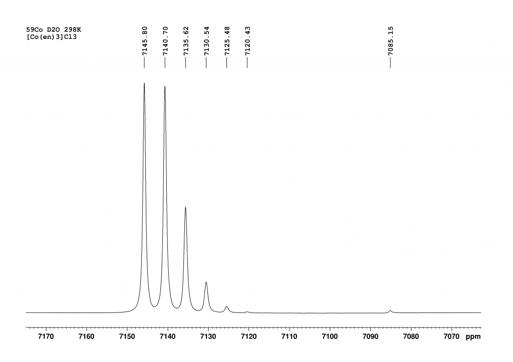
Figure 2: 59Co NMR spectrum of [Co(en)3]Cl3 and D2O. Recorded approximately 30 minutes after sample preparation on a 700 MHz spectrometer at 298 K. Seven isotopomers can be seen (see discussion).
As expected, the spectrum had a very good signal to noise ratio but instead of the expected singlet, 7 peaks were visible. My first thought was that the solid we had dissolved was heavily contaminated. I was about to dispose of the sample when I noticed that the 6 peaks at low field were almost exactly 5 ppm away from their neighboring peaks. This could not be a coincidence and could not be explained by random decomposition products or impurities. However, I definitely thought the peak at high field (7085 ppm) was an impurity – a clear misjudgment. About 24 hours after the first measurement, I wanted to look at the same sample again and repeated the measurement. This time I was really amazed by the mesmerizing spectrum I got.
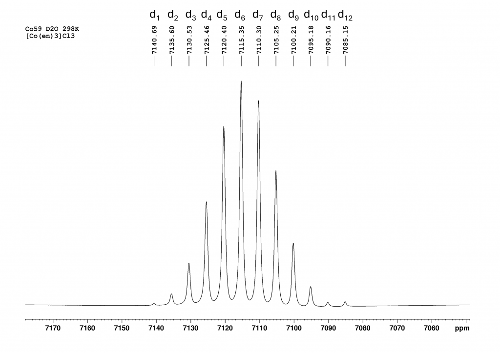
Figure 3: 59Co NMR spectrum of the isotopomers of [Co(en)3]Cl3 in D2O. Recorded approximately 24 hours after sample preparation on a 700 MHz spectrometer at 298 K.
Now 12 peaks can be observed at intervals of 5 ppm and it can be seen that the signal at 7085 ppm also belongs to this ensemble of peaks. After a brief literature search, it quickly became clear what was going on here. The 12 peaks from low to high field are the isotopomers d1 to d12-[Co(en)3]3+, which were formed by H/D exchange of the NH2 protons. The signal of the non-deuterated complex (d0) has already disappeared.By integrating the CH2 protons of the ethylenediamine ligands against the remaining NH protons, the degree of deuteration can be determined at this point, which corresponds to nearby 50%. The isotope effect caused by the successive deuteration of the NH2 groups has been known since the 1980s and the kinetics of this reaction were already studied in detail at that time by Harris et al. with the aid of 59Co NMR.3 At the time, the authors only had access to a 100 MHz NMR spectrometer. The analysis of the spectra therefore had to be carried out using deconvolution. From this perspective, the kinetic analyses described are all the more impressive. In a publication by Zardrozny et al. from 2022, it was proposed to use this H/D exchange for a molecular thermometer.4
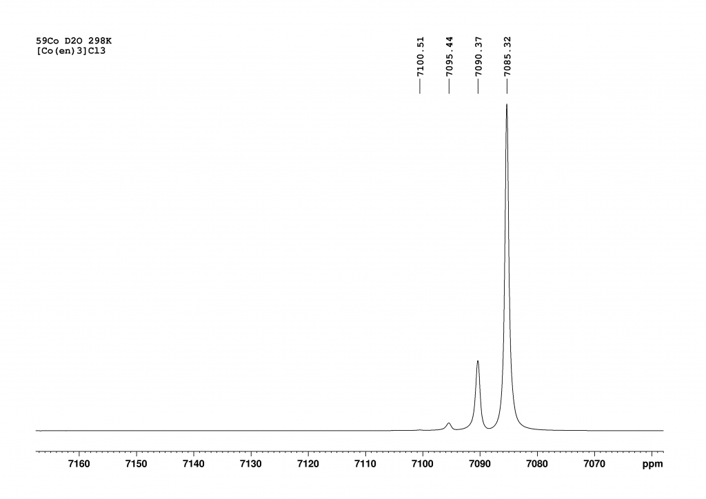
Figure 3: 59Co NMR spectrum of the isotopomers of [Co(en)3]Cl3 in D2O at equilibrium. Recorded approximately 1 week after sample preparation on a 700 MHz spectrometer at 298 K.
After approximately 1 week, only 4 peaks can finally be observed, with the peak at 7085 ppm (d12-complex) now dominant. The degree of deuteration is now at 98%, which agrees very well with the literature value of Harris et al. who observed the complexes d12 to d10 at equilibrium. With our much more powerful spectrometer, we also see the d9-complex at 7100.5 ppm. Due to the protons in solution, a small proportion of NH species always remains in equilibrium. While I was working on the spectra, the question arose as to why there should only be 13 peaks (d0 to d12). In fact, there should be many more, because for most isotopomers (except d0, d1, d11 and d12) there are stereoisomers that should increase the number of peaks. For example, if we consider only the case d2, there are 3 stereoisomers (see Figure 4).
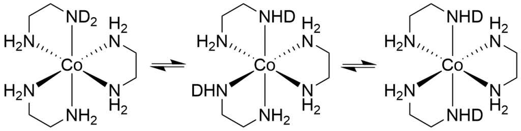
Figure 4: Stereoisomers of d2-[Co(en)3]3+
In the first there is simply an ND2 group, in the second the two NHD groups are in the cis position and in the third in the trans position. Since we only see one signal for these 3 isomers in the 59Co spectrum, I assume that there is a very fast intramolecular H/D exchange, so that the spectrometer only shows an averaged signal over the chemical shifts of the 3 isomers. This can then also be assumed for all other isotopomers. This is probably also the reason why the signals always shift by 5 ppm with each additional deuterium. Because it is not the position of the deuterium atoms but only their number that determines the chemical shift.
Whenever I think I have seen everything there is to see in the field of NMR spectroscopy, I come across something unexpected, as in this case.
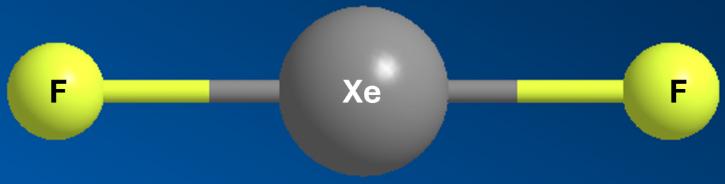
XeF2 is a small but spectacular molecule and therefore a good starting point for this blog. Since its first synthesis in 1962 by Rudolf Hoppe1, this compound has been extensively studied for its chemical and spectroscopic properties. I was lucky enough to have an NMR sample of XeF2 in CD3CN brought to me by one of our Ph.D. students, who funnily enough has the same last name as the discoverer of the molecule. The first thing I did was to measure the 129Xe spectrum.
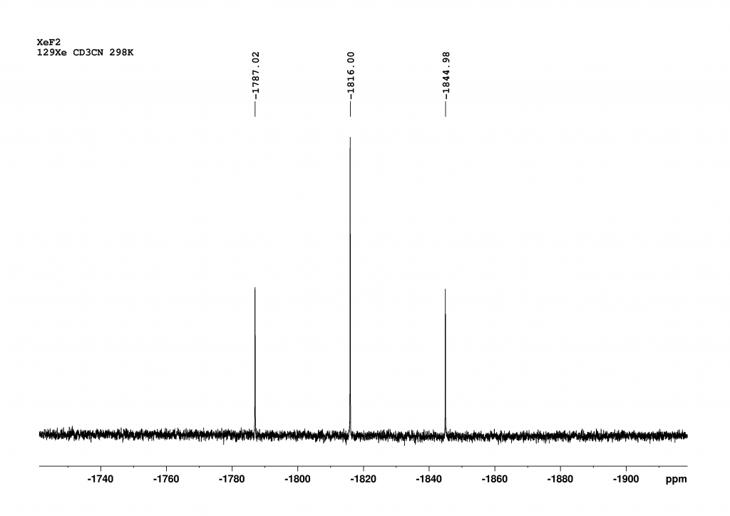
Figure 1: NMR of XeF2 measured in CD3CN at 298 K with a 700 MHz NMR spectrometer (128 Scans, AQ= 4 min, FWHM=18 Hz). Chemical shifts are given relative to XeOF4 (= 0 ppm).
The measurement was kept as short as possible to ensure that the solution did not contain any decomposition products. XeF2 is so reactive that it slowly degrades through the glass wall of the tube2. However, this great caution was not necessary as the lifetime of XeF2 in CD3CN is more than sufficient. In addition, the receptivity of 129Xe is 33 times higher than that of 13C, resulting in a good signal-to-noise ratio (SNR) even with short measurement times.
129Xe spectrum
Although the sample was very precisely tempered to 298 K, the chemical shift found of -1816 ppm will have a small error as we had no reference. However, the fact that this error is not very large can be seen from the correlability of our data in CD2Cl2 with literature values. For example, the chemical shift in CD2Cl2 at 263 K was given as a value of -1850 ppm. The authors state that the chemical shift changes by -0.64 ppm/K.3 Extrapolated to 298 K, this means that a chemical shift of -1874 ppm is to be expected, which is in excellent agreement with the value of -1875 ppm that we found. The significant difference in chemical shifts between CD3CN and CD2Cl2 demonstrates the sensitivity of 129Xe to its environment. As expected, the coupling with the fluorine atoms results in a triplet. The magnitude of the 1JXeF coupling constant is 5645 Hz in CD3CN and 5600 Hz in CD2Cl2, which falls within the range of values reported in the literature.4,5 The solvent therefore also has a noticeable effect on the coupling constant. As always, only the magnitude of the coupling constant can be obtained from the 1D spectrum. In fact, the 1JXeF coupling constant is negative because, as theorists have shown, all Ramsey terms contributing to the coupling constant are negative.6
19F Spectrum
To be honest, I only included the 19F spectrum for the sake of completeness and didn’t expect any surprises. At first glance, it looks as expected.
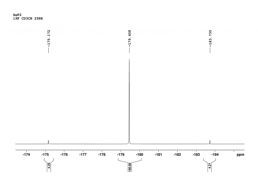
Figure 2: 19F spectrum of XeF2 in CD3CN measured at 298 K with a 700 MHz spectrometer (1 Scan, no dummy scans). The spectrum is shown with reference to CFCl3 (= 0 ppm).
There are two signals in the spectrum. The middle peak shows the chemical shift of all the fluorine atoms that are not bound to 129Xe and 131Xe (52.3% of all Xe atoms). The signals of the 19F atoms bound to 131Xe disappear due to very fast relaxation in the baseline (see below). The two outer peaks are a doublet (1JXeF = 5645 Hz) resulting from the coupling of the fluorine atoms bound to 129Xe (26.4% natural abundance). At this point a detective story begins as the integrals obviously do not reflect the natural abundances of the isotopomers. According to the integrals in the spectrum, the natural abundance of 129Xe should be only 7.8%. To rule out the possibility of relaxation effects influencing the integrals, the spectrum was recorded with only one scan and without dummy scans. We waited 5 minutes before the scan. Even if the 19F atoms were excited when setting up the sample (determining the receiver gain), this time is more than sufficient to reach equilibrium, given that the T1 time of the 19F atoms in the solvent CD3CN is approximately 10 seconds.7 I discussed this with a very experienced colleague, who said that the 129Xe in the sample could be depleted, but we had no idea why. During my literature search for 19F measurements on XeF₂, I came across a very interesting paper by Jokisaari and Schrobligen et al.8 They had carried out measurements in CD3CN at -16°C, which significantly improved the resolution of the 19F spectrum. We therefore repeated the 19F measurement at -25°C in CD3CN, which enabled us to differentiate most of the isotopomers, as described by the authors.
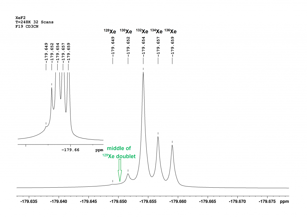
Figure 3: This is a section of the 19F spectrum of XeF₂ at -25°C in CD₃CN. The central signal, composed of the peaks of the isotopomers 128Xe, 130Xe, 132Xe, 134Xe and 136Xe, is shown.
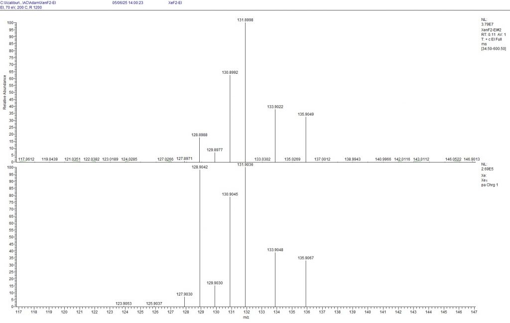
Compared to the spectrum at 25°C (Figure 2), five isotopomers can now be distinguished in the central signal area. Figure 3 shows that the intensity of the signals approximately corresponds to their natural abundances [126Xe (0.09%), 128Xe (1.9%), 130Xe (4.1%), 132Xe (26.9%), 134Xe (10.4%), 136Xe (8.9%)]9. The 129XeF₂ doublet lies outside the section. The centre of the doublet is calculated to be almost exactly between the peaks of 128XeF2 and 130XeF2. The associated integral still does not correspond to the natural abundance of 129Xe. The abundance is only 7.8% here, too. The sequence of chemical shifts correlates well with the mass of the isotopomers. The greater the mass, the stronger the high-field shift of the peak. An increase in the mass number by 2 leads to a primary isotope shift of -2 to -3 ppb. To solve the mystery of the isotopomers, I asked the PhD student who had prepared the sample for me (thanks Axel!) to measure a mass spectrum of the solid XeF2. The following figure shows the result.
Figure 4: Mass spectrum of XeF2 (top) measured with EI (70 eV). The isotope distribution of Xe+ is shown. The natural isotope distribution is shown below for comparison (To enlarge the image, point to the image with the mouse and press the Ctrl key twice.)
The mass spectrometric measurements show that all isotopes from 128Xe to 131Xe are depleted, while all isotopes from 132Xe to 136Xe are enriched. According to the measurement, only 6.9% of 129Xe is present in the mixture, which agrees surprisingly well with the NMR measurements presented above. The results of the mass spectrometry compared to the NMR results also indicate that the 19F signal of 131XeF2 is not recognisable, but was probably integrated as a very broad peak among the other signals in the -179.65 ppm range.
I did a little research on the internet about the enrichment of 129Xe and it seems that 129Xe is indeed enriched on a large scale for medical purposes. It is used very successfully as hyperpolarised 129Xe in MRI examinations of the human lung.10 We contacted the XeF₂ vendor and provided them with the measurement results. They were unaware that their product did not have the natural distribution of xenon isotopes, which could cause major spectroscopic problems for their customers. I am sure the vendor will ask his xenon supplier some questions…