25 years ago, Peringer et al. published a paper entitled “1J(199Hg199Hg) values of up to 284 kHz in complexes of [Hg–Hg]2+ with crown
ethers: the largest indirect coupling constants”.1
It reports on the extremely large scalar coupling constants between non-equivalent directly bonded mercury atoms. Unfortunately, the communication was not followed by a full paper.2 In this post I would like to address some questions that have remained unanswered and explain in more detail how the authors calculated the coupling constants of the mercury atoms.
Perhaps this will motivate someone to repeat the experiments in order to clarify the questions. I think there is still plenty of room for interesting discoveries.
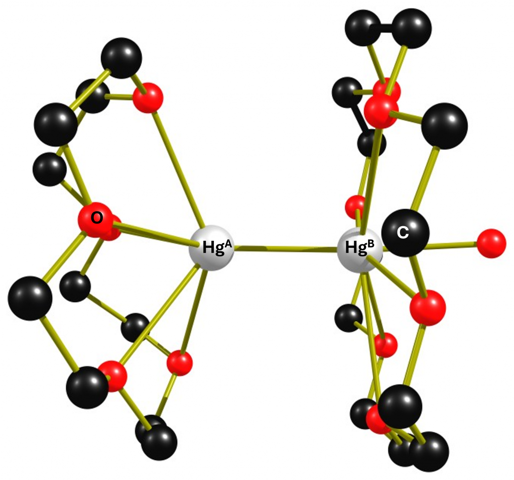
The reaction of a simple Hg2+ salt with elemental mercury and subsequently with the ether 18-crown-6 leads after crystallization from dichloromethane to the complex cation {[Hg2(18-crown-6)2(dmso)(μ-dmso)]}24+(complex 1). The structure of this cation is shown below.
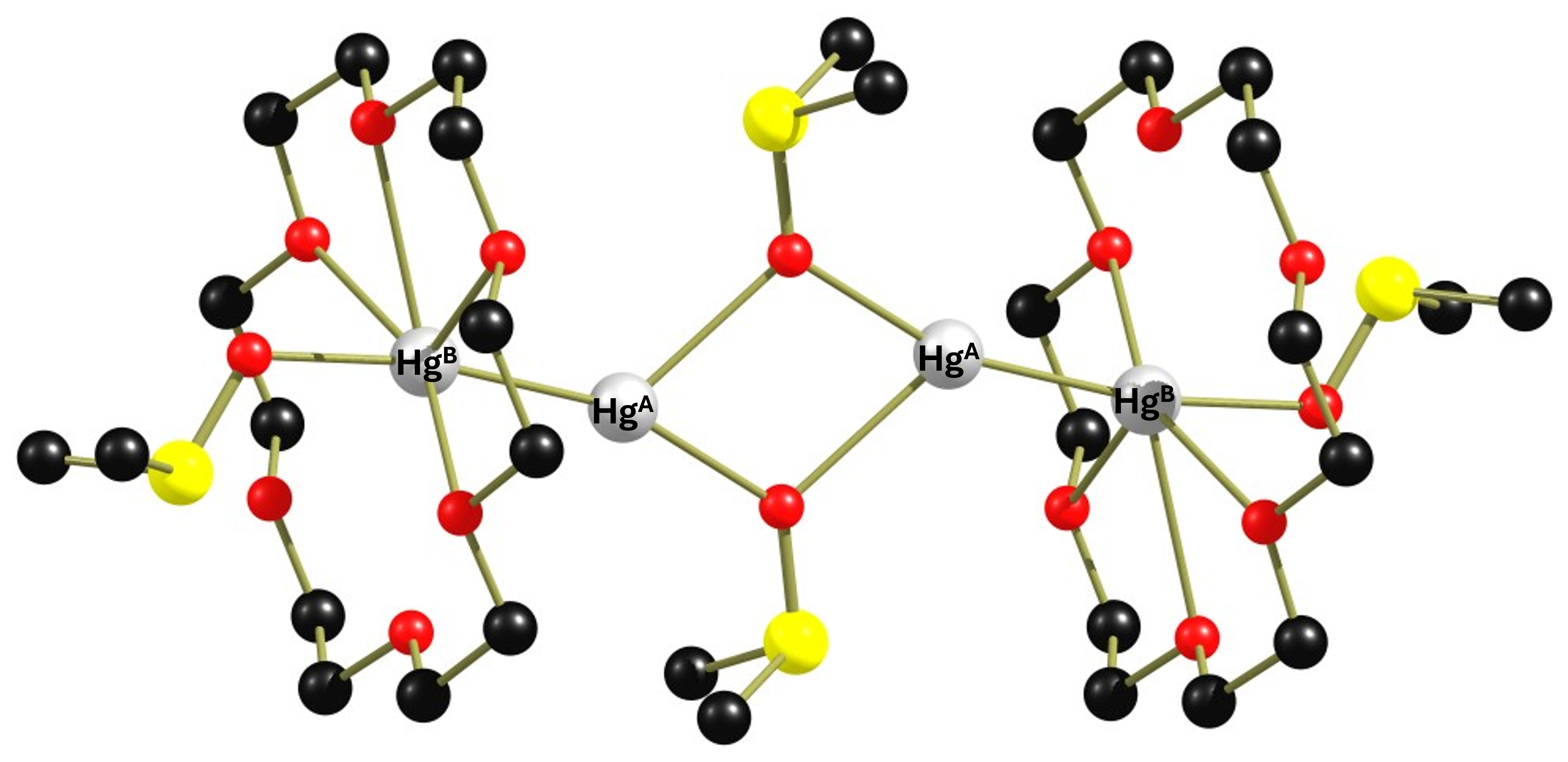
The dimeric complex 1 is highly interesting because it contains two non-equivalent Hg(+I) atoms that are linked to each other via an Hg-Hg bond and will therefore couple with each other in the 199Hg NMR spectrum. Before we look at the NMR spectrum of the compound, I would like to discuss a detail in the structure of complex 1 that is important for the spectra. Of the six Hg-O distances, four are in the range of 2.7 Å to 2.8 Å and two are in the range of 3.0 Å, which is already larger than the sum of the van der Waals radii of mercury and oxygen. Therefore, in figure 1, two oxygen atoms have no coordinative bond to the mercury atom. The original paper was more generous. In any case, the large differences in the Hg-O distances indicate that the crown ether binds fluxionally. Unfortunately, neither 13C nor 1H NMR data were given in the paper, so no statement can be made about the dynamic behaviour of the ligand. Only one 199Hg spectrum (reference HgO/HClO4) was recorded at 243 K in non-deuterated dichloromethane, showing 4 signals.
Insert: NMR spectra of AB spin systems
If the coupling constant JAB of two atomic nuclei A and B is in the range of the difference between their Larmor frequencies (Δν=νA-νB), the phenomenon of strong coupling occurs and this is referred to as an AB spin system. If the difference between the Larmor frequencies is significantly greater than JAB (at least more than 10 times), this is referred to as a first-order spectrum and an AX spin system is present, which shows two simple doublets in the spectrum according to the n+1 rule. The NMR spectrum of an AB spin system typically looks like the one shown in the next figure.
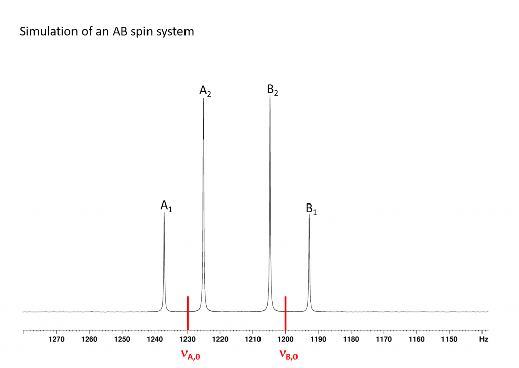
The spectrum shown is typical of an AB spin system. Compared to the AX spin system, the two doublets are distorted. The inner transitions (A2 and B2) are much more intense than the outer transitions (A1 and B1). It should also be noted that the Larmor frequencies (νA,0 and νB,0) of the nuclei are no longer in the centre of the doublets, but are shifted towards the more intense transition. As Δν becomes smaller, peaks A1 and B1 become smaller and A2 and B2 become larger. In terms of the 199Hg spectra discussed below, this means that the A1 and B1 transitions become so small that they are lost in the noise of the spectra, so that only the A2 and B2 peaks can be detected. At first sight, one might think that the coupling constant JAB can no longer be determined. After all, it is calculated very simply from the difference νA,1-νA,2 or νB,2-νB,1. However, if you know the position of νA,0 and νB,0, there is another way to calculate the coupling constant JAB. The corresponding equation is
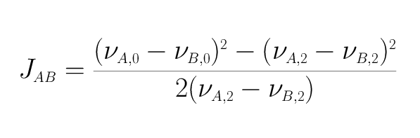
It can be derived from the basic equations3 that describe the frequency positions in an AB spin system.
199Hg NMR spectrum of complex 1
The spectrum of complex 1 is not shown in the original paper. However, it can be reconstructed from the given data by means of simulation. The spectrum was measured at 243 K in CH2Cl2 at 53.63 MHz (i.e. on a 300 MHz NMR spectrometer). The chemical shift of HgA is 944 ppm and that of HgB (complexed to 18-crown-6) is 435 ppm. At this point, I would like to point out that the authors do not explain how they arrived at this signal assignment. The coupling constant 1JHgHg is an incredible 220300 Hz (± 790 Hz). The spectrum then looked something like this:
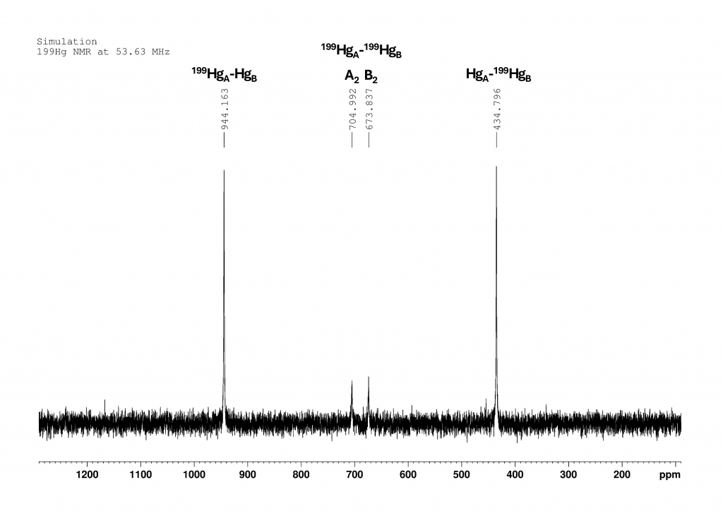
The two large peaks show the signals of 199HgA bound to a non-active Hg (944 ppm) and 199HgB bound to a non-active Hg. The two small peaks in the center belong to the two doublets that are formed by the coupling of two 199Hg atoms. They correspond to peaks νA,0 (705 ppm) and νB,0 (674 ppm) from Figure 2.
There are 7 stable mercury isotopes. Only the isotope 199Hg (natural abundance 16.94% 5) is accessible in liquid using NMR spectroscopy. If we look at complex 1, there are 10 isotopomers to consider for the spectrum.
In the following list, all 199Hg atoms are labeled with Hg and all other Hg isotopes are summarized under the symbol Hg.
List of the isotopomers containing of complex 1:
Isotopomer 1 abundance 47.60%
[(dmso)(18-crown-6)HgB-HgA(μ-dmso)2HgA-HgB(18-crown-6)(dmso)]4+
Isotopomer 2 abundance 19.41%
[(dmso)(18-crown-6)HgB-HgA(μ-dmso)2HgA-HgB(18-crown-6)(dmso)]4+
Isotopomer 3 abundance 19.41%
[(dmso)(18-crown-6)HgB–HgA(μ-dmso)2HgA-HgB(18-crown-6)(dmso)]4+
Isotopomer 4 abundance 3.96%
[(dmso)(18-crown-6)HgB–HgA(μ-dmso)2HgA-HgB(18-crown-6)(dmso)]4+
Isotopomer 5 abundance 3.96%
[(dmso)(18-crown-6)HgB-HgA(μ-dmso)2HgA-HgB(18-crown-6)(dmso)]4+
Isotopomer 6 abundance 1.98%
[(dmso)(18-crown-6)HgB–HgA(μ-dmso)2HgA-HgB(18-crown-6)(dmso)]4+
Isotopomer 7 abundance 1.98%
[(dmso)(18-crown-6)HgB-HgA(μ-dmso)2HgA–HgB(18-crown-6)(dmso)]4+
Isotopomer 8 abundance 0.81%
[(dmso)(18-crown-6)HgB–HgA(μ-dmso)2HgA–HgB(18-crown-6)(dmso)]4+
Isotopomer 9 abundance 0.81%
[(dmso)(18-crown-6)HgB–HgA(μ-dmso)2HgA-HgB(18-crown-6)(dmso)]4+
Isotopomer 10 abundance 0.08%
[(dmso)(18-crown-6)HgB–HgA(μ-dmso)2HgA–HgB(18-crown-6)(dmso)]4+
Only isotopomer 1 does not give a NMR signal. Since the measured 199Hg NMR spectrum provides only four signals of very different intensities, it is reasonable to conclude that 199Hg atoms not directly bound to another 199Hg atom exhibit a single resonance for both HgA and HgB. These resonances correspond to the νA,0 and νB,0 positions shown in Figure 2. The intensity of these signals is directly proportional to the abundance of 199Hg in positions A and B, respectively.6 We then expect the intensity ratio of the four peaks to be approximately 5:1:1:5, with roughly comparable line widths in the spectrum shown in Figure 3.
Dinuclear complexes [(15-crown-5)Hg-Hg(18-crown-6)(L)]2+ (L=dmso, MeOH, H2O)
When complex 1 is reacted with two equivalents of 15-crown-5 in CH₂Cl₂, it degrades to form the dinuclear complex [(15-crown-5)Hg-Hg(18-crown-6)(dmso)]2+ (2). This cocrystallises with complex [(15-crown-5)Hg-Hg(18-crown-6)(H2O)]2+ 3 when an attempt is made to isolate it. However, it is possible to spectroscope complex 2 cleanly in solution. I have isolated the structure of complex 3 from the corresponding cif file, which is shown below. I have dispensed with complex 2 because some of the carbon atoms in it are so strongly disordered that its representation becomes very confusing.
All distances are in the range of the sum of the van der Waals radii of oxygen and mercury, but the high variance with differences in the distances of 0.3 Å and 0.8 Å, respectively, strongly indicate that the crown ethers in solution should show a pronounced fluxional behavior. Unfortunately, the authors do not provide any 1H or 13C NMR data, so the dynamic behaviour of the ligands cannot be verified.
The 199Hg NMR spectrum of complex 2 in CH2Cl2 at 223K is analogous to the spectrum of complex 1 (Figure 2). It does not add much value, but I simulated and plotted it anyway so that the reader does not have to scroll up constantly.
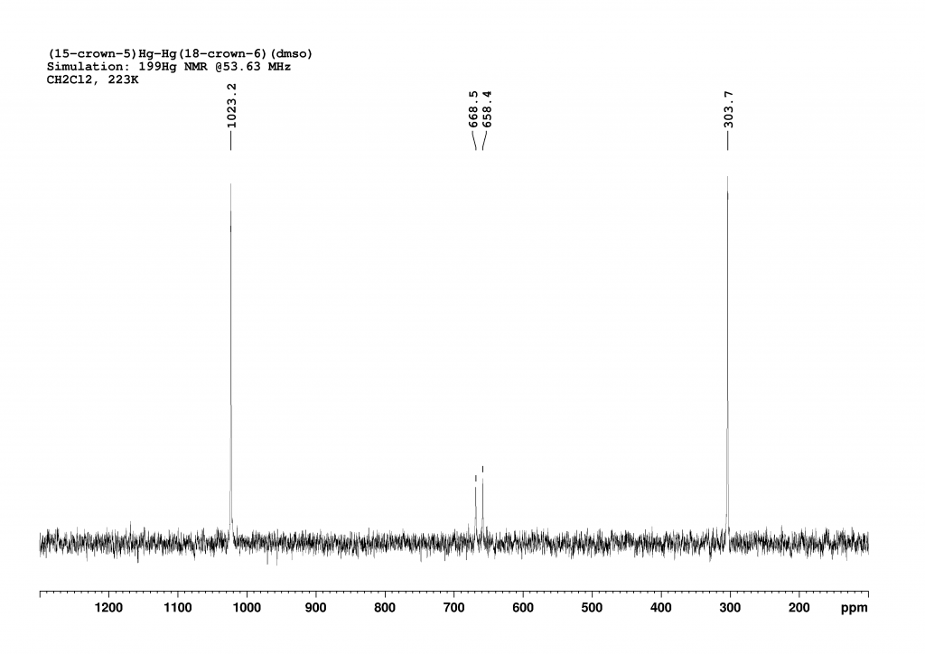
In this case, the coupling constant is calculated as 263200 Hz (±590 Hz).
But that’s not the end of the story. The record-breaking result is obtained when complex 1 is dissolved in methanol. In this case, an equilibrium between [(15-crown-5)Hg-Hg(18-crown-6)(dmso)]2+ 2 and [(15-crown-5)Hg-Hg(18-crown-6)(MeOH)]2+ 4 forms in the solution. Unfortunately, the authors do not comment on the position of this equilibrium. Nevertheless, analysis of the 199Hg NMR spectrum of this mixture reveals a 1JHgHg coupling constant of 284100 Hz (±860 Hz) in 4, which is the highest coupling constant recorded to date. Unfortunately, 4 could not be crystallised. Instead, mixed crystals of 2 and 3 were obtained. The water had diffused from the air into the methanol during crystallisation, which did not take place under protective gas.
Loose ends
It is in the nature of a short communication that not all aspects of chemistry and spectroscopy can be covered. Since the large coupling constants reported are of great importance for NMR spectroscopy, I would like to conclude by pointing out a few questions that should be answered in the future.
1. In any case, the measurements should be repeated using a modern spectrometer and a more common standard in deuterated solvents.
2. In all 199Hg NMR spectra, the mercury signal bound to 18-crown-6 should appear at a low frequency of approximately 300–400 ppm. However, the paper does not explain how this assignment was made. I suspect that the authors also produced the compound [(18-crown-6)Hg-Hg(18-crown-6)(dmso)]2+, in which both Hg atoms are complexed by 18-crown-6, which would make the assignment much more reliable.
3. Does complex 1 split into dinuclear complexes in solution, or is it tetranuclear?
This question must be asked when comparing the 199Hg chemical shifts of the complex with those of the dinuclear complexes 2 and 4. The differences are strikingly small, which is surprising given their quite different structures. This question can be answered quickly using DOSY measurements.
4. The dynamics of the ligands should also be investigated using temperature-variable 1H and 13C spectra. The solid-state structures suggest that the ligands may exhibit fluxional behaviour in solution.
5. Could complex 1 be cleaved with other ligands L (e.g. PR3) to generate further type [(L)Hg-Hg(18-crown-6)(dmso)]2+ complexes and investigate the dependence of the coupling constant on L in more detail?
References:
- https://doi.org/10.1039/B007581G ↩︎
- This is not about scolding authors. I think the authors’ discovery is great and I’m glad they reported it! ↩︎
- James Keeler, Understanding NMR Spextroscopy, 2nd Ed., John Wiley & Sons , Ltd.
Please note that Prof Keeler works very precisely with negative Larmor frequencies, so all frequency positions given in the book must be multiplied by -1 to obtain them in the usual representation, which is also used in this post. ↩︎ - https://doi.org/10.1039/B007581G ↩︎
- Mercury Isotopes – List and Properties ↩︎
- Example for the calculation of the relative intensity I of the peak of νA,0 for HgA. The isotopomers 3, 5, 6 and 9 must be taken into account:I=19.41/4+3.96/4+1.98/2+0.81/4=7.035. The same result is obtained for νB,0, of course. ↩︎